Computing Spectrograms

Code

Today's code distribution is available here. It contains a skeleton file for today's code, as well as four different tunes to analyze.

So far in the course, we have done a lot of analysis using the Fourier transform of an entire signal.

Recall that a subset of samples in time (e.g., n to n+5, where N\geq 5) contributes to all Fourier coefficients (i.e., a_0 to a_{N-1}). Similarly, a subset of Fourier series coefficients (e.g., a_0 to a_3) contributes to all samples in time (i.e., from n=0 to n=N-1). In other words, "local" information in one domain becomes "global" information in the other domain.

Therefore, sudden changes and local variations of the signal (such as the beginning and end of notes in a piece of music) can be challenging to detect when directly using Fourier transform. For instance, music is composed of different notes, which are of different frequencies at different times.

To mitigate these drawbacks and enhance our ability to visualize how the frequency characteristics of a signal vary with time, we'll introduce a new notion: the short-time Fourier transform. This transform is a compromise between time- and frequency-domain representations, detemining the sinusoidal frequency and phase content of local sections of a signal as it changes over time.

We start with a signal x[n]. We divide this signal into analysis windows of length N, with beginning times spaced s samples apart, such that window i contains samples x[i\times s] through x[i\times s + N - 1] (inclusive). This "windowing" process is described in the picture below:

The short-time Fourier transform consists of a sequence of Fourier transforms X_i[k], with one transform for each analysis window.

You may assume that a function called fft has been defined for you in the box below (you do not need to include your definition of fft).

def stft(x, window_size, step_size, sample_rate): # return a Short-Time Fourier Transform of x, using the specified window # size and step size. # return your result as a list of lists, where each internal list # represents the DFT coefficients of one window. I.e., output[n][k] should # represent the kth DFT coefficient from the nth window. pass

Loading...

As we have seen in the past, the frequency (in Hz) associated with a particular value of k depends on the value N. Fill in the definition of the k_to_hz and hz_to_k functions to provide a way to map between the two.

We'll also be interested to convert our horizontal axis to units of time (seconds). Fill in the definition of timestep_to_seconds as well.

Paste your code for these functions into the box below to check for correctness:

def k_to_hz(k, window_size, step_size, sample_rate): # return the frequency in Hz associated with bin number k in an STFT with # the parameters given above. pass def hz_to_k(freq, window_size, step_size, sample_rate): # return the k value associated with the given frequency in Hz, in an STFT # with the parameters given above, rounded to the nearest integer. pass def timestep_to_seconds(i, window_size, step_size, sample_rate): # return the real-world time in seconds associated with the center of the # ith window in an STFT using the parameters given above, rounded to the # nearest .01 seconds. pass

Loading...

The spectrogram of a signal is defined to be the squared magnitude of the STFT. Write a function that takes in the output of your stft function (among other parameters) and generates the spectrogram of the signal.

Conventionally, the horizontal axis in a spectrogram represents time. As such, your spectrogram function should return a 2-d array (list of lists) that is indexed first by k, and then by i.

To help with this process, write a function called transpose, which takes in a 2-d array and returns a new 2-d array representing its transpose.

Write these functions (you may wish to start with transpose) and enter them in the box below to check your result:

def transpose(x): # return the transpose of the input, which is given as a list of lists pass def spectrogram(X, window_size, step_size, sample_rate): # X is the output of the stft function (a list of lists of DFT # coefficients) this function should return the spectrogram (magnitude # squared of the STFT). # it should be a list that is indexed first by k and then by i, so that # output[k][i] represents frequency bin k in analysis window i. pass

Loading...

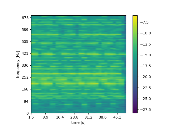
We have provided a function called plot_spectrogram, which can be used to display the result. As an example, here is the spectrogram of a small piece of a current top 40 song, generated using the functions from this lab:

Look at the code for plot_spectrogram to get a sense of how it behaves.

Why do we only need to plot through N/2? Why not plot all N frequency bins? How could we zoom in to focus on just lower frequencies.

Check In:
Choose any of the .wav files in this week's distribution, and plot its spectrogram. Explain the important features of your plot.

Ask for Checkoff Loading...

Plot the spectrogram of each of the tunes in the distribution. What does the spectrogram tell you about what is happening in the tune? Can you predict anything about the tune, based on the spectrogram?

How do the parameters window_size and step_size affect your results? Which combination gives the most insightful visualization of the tune and why?

Please upload a single pdf file that contains your answers to all parts of this problem:

Select File No file selected

Loading...

If you have the time and interest, convert a portion of a real song to a mono wave file and plot its spectrogram. What features in the spectrogram arise from what features in the song? How do the window_size and step_size parameters affect the output?

On systems with ffmpeg installed, you can use the following to convert to the proper format, where your_file is an input file, t1 is a starting time of the clip you want to encode (in seconds), dt is the length of the clip you want to encode (in seconds), and output.wav is the name of the file you want to save (it should end with .wav):

$ ffmpeg -i your_file -ss t1 -t dt -ac 1 -ar 44100 output.wav

For example, to take a 10-second clip of a file, starting at the 30-second mark, and convert it to the proper format, you could use:

$ ffmpeg -i havana.mp3 -ss 30 -t 10 -ac 1 -ar 44100 havana.wav